

Linear Regression: From Theory to Implementation
Linear regression models the relationship between one or more input variables and a continuous target. This article develops a univariate linear regression model from first principles, derives the gradient descent updates, and implements the complete training procedure with NumPy.
The discussion uses a small housing-price dataset so that each step can be inspected directly. Here, one unit of house size represents 1,000 square feet, and one unit of price represents 1,000 dollars.
This article reorganizes notes based on Andrew Ng’s Supervised Machine Learning: Regression and Classification course. The explanations and implementation are independently written and simplified for study purposes.
1. Problem formulation
In supervised learning, a model learns a mapping from an input $x$ to a known target $y$. Regression problems predict continuous values such as prices, temperatures, or demand. Classification problems, by contrast, predict discrete classes.
The example dataset contains two observations:
| House size $x$ (1,000 ft²) | Price $y$ (1,000 USD) |
|---|---|
| 1.0 | 300.0 |
| 2.0 | 500.0 |
For univariate linear regression, the prediction function is
\[f_{w,b}(x) = \hat{y} = wx+b,\]where:
- $x$ is the input feature;
- $y$ is the observed target;
- $\hat{y}$ is the model prediction;
- $w$ is the weight, or slope;
- $b$ is the bias, or intercept.
The two observations lie exactly on the line
\[\hat{y}=200x+100.\]Consequently, a house of size $x=3$ is predicted to cost 700 thousand dollars.
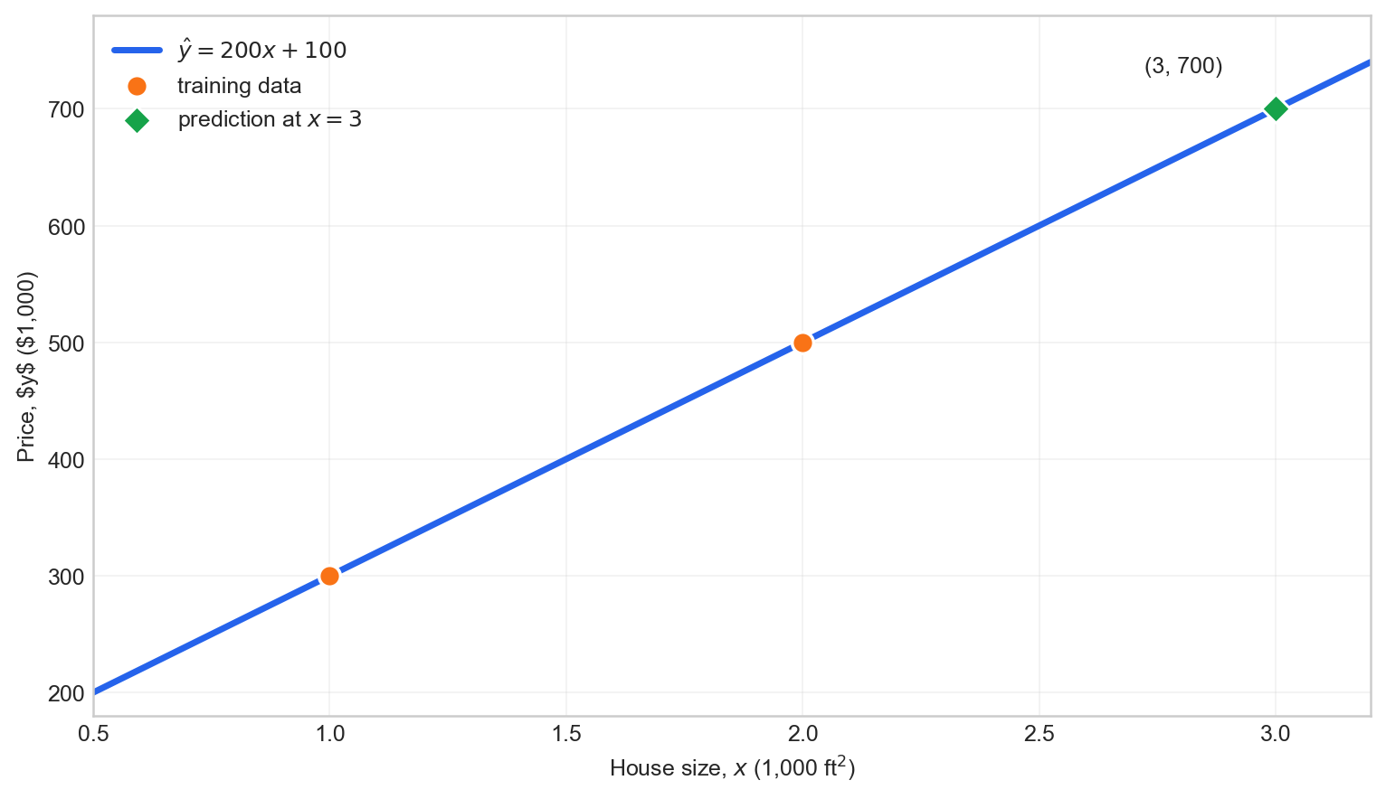
In practical datasets, observations rarely lie exactly on a straight line. The objective is therefore to find the values of $w$ and $b$ that produce the smallest overall prediction error.
Why begin with one feature?
I initially found the notation more difficult than the model itself. Writing $f_{w,b}(x)$, $x^{(i)}$, and $\hat{y}^{(i)}$ makes a straight line appear more complicated than it is. Reducing the problem to one feature made the role of each symbol visible:
- choose one observation $x^{(i)}$;
- substitute it into $wx+b$;
- compare the prediction with $y^{(i)}$;
- repeat the comparison for every observation.
The superscript $(i)$ is an index, not an exponent. Thus, $x^{(2)}$ means the second observation rather than $x$ squared. This distinction becomes important as soon as a summation appears in the cost function.
The parameters also have concrete geometric meanings. Changing $w$ rotates the line, whereas changing $b$ shifts the entire line vertically. Training a linear model is therefore equivalent to moving and rotating a line until it fits the observations as well as possible.
For the two-point example, the parameters can be obtained directly:
\[w=\frac{500-300}{2-1}=200,\] \[b=300-200\times1=100.\]This direct solution is useful as a reference. It allows the result of gradient descent to be checked against a known answer. The purpose of gradient descent in this example is not that two points require numerical optimization, but that the same optimization structure extends to models for which a convenient manual solution is unavailable.
2. Cost function
For an individual observation $i$, the residual is
\[e^{(i)} = f_{w,b}(x^{(i)})-y^{(i)}.\]Positive and negative residuals would cancel if they were added directly. Squaring them avoids cancellation and penalizes large errors more strongly. For $m$ observations, this article uses the following objective:
\[J(w,b)=\frac{1}{2m}\sum_{i=1}^{m}\left(f_{w,b}(x^{(i)})-y^{(i)}\right)^2.\]This is one half of the mean squared error (MSE). The factor $1/2$ does not change the minimizing parameters; it only cancels the factor $2$ that appears during differentiation.
It is also useful to distinguish an individual loss from the aggregate cost. The squared error of one observation describes how wrong one prediction is. $J(w,b)$ averages that error over the complete training set and is the quantity optimized during batch gradient descent. The terms are often used interchangeably in informal explanations, but keeping the distinction made the later equations easier for me to follow.
For example, suppose the predictions are $[100, 400, 500]$ and the targets are $[200, 300, 500]$. Then
\[J=\frac{(-100)^2+(100)^2+0^2}{2\times3}=3333.33.\]A smaller value of $J$ indicates a better fit to the training data. A value of zero means that every prediction matches its target exactly.
Why square the residuals?
| Squaring is not the only way to prevent positive and negative residuals from cancelling. Mean absolute error uses $ | \hat{y}-y | $ instead. The squared-error objective is particularly convenient here for two reasons: |
- it is differentiable everywhere and produces a simple gradient;
- large residuals receive a disproportionately large penalty.
The second property is both useful and potentially undesirable. It encourages the model to correct large mistakes, but it also makes the objective sensitive to outliers. The choice between squared and absolute error should therefore follow the characteristics of the data rather than habit.
How the parameters become a surface
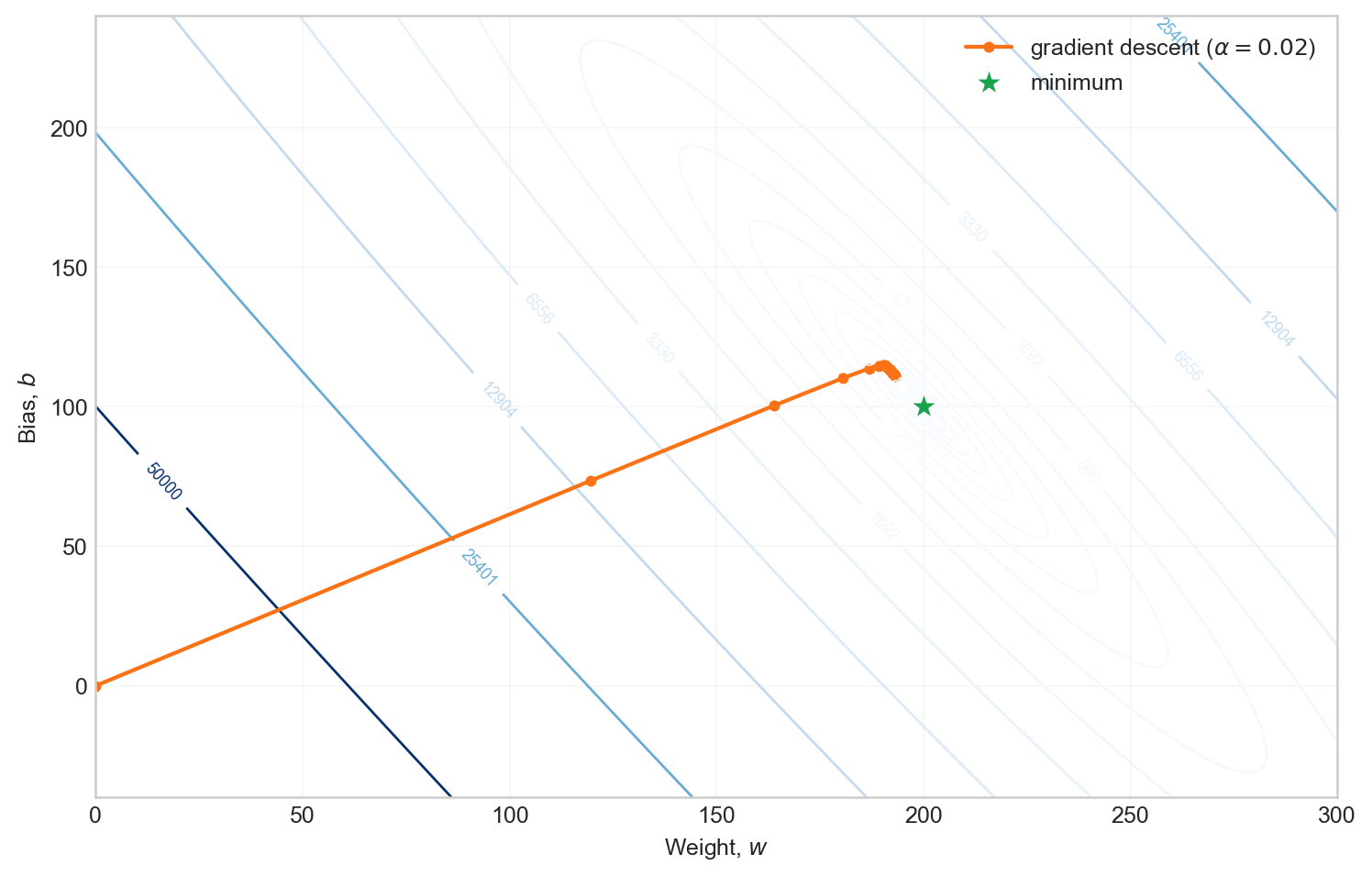
For fixed $w$ and $b$, the model produces one scalar cost. If only $w$ is varied while $b$ is fixed, $J(w,b)$ can be drawn as a two-dimensional bowl-shaped curve. If both parameters are varied, the cost becomes a surface over the $(w,b)$ plane. A contour line connects parameter pairs with the same cost, just as a contour on a map connects locations with the same elevation.
The squared-error objective for linear regression is convex. Therefore, it has no suboptimal local minima: every local minimum is also a global minimum. The contour plot below shows the cost associated with different combinations of $w$ and $b$.
3. Gradient descent
Gradient descent iteratively adjusts the parameters in the direction that reduces the cost. With learning rate $\alpha>0$, the updates are
My first intuition was to increase or decrease $w$ by an arbitrary amount after looking at a cost curve. That approach does not scale: the correct direction depends on the current position, and the size of an appropriate step changes along the surface. The derivative resolves the first issue by describing the local direction and steepness. The learning rate controls how much of that proposed movement is taken.
\[w \leftarrow w-\alpha\frac{\partial J}{\partial w},\] \[b \leftarrow b-\alpha\frac{\partial J}{\partial b}.\]For univariate linear regression, the partial derivatives are
\[\frac{\partial J}{\partial w} =\frac{1}{m}\sum_{i=1}^{m} \left(f_{w,b}(x^{(i)})-y^{(i)}\right)x^{(i)},\] \[\frac{\partial J}{\partial b} =\frac{1}{m}\sum_{i=1}^{m} \left(f_{w,b}(x^{(i)})-y^{(i)}\right).\]Derivation
Substituting $f_{w,b}(x^{(i)})=wx^{(i)}+b$ into the cost function gives
\[J(w,b)=\frac{1}{2m}\sum_{i=1}^{m} \left(wx^{(i)}+b-y^{(i)}\right)^2.\]Applying the chain rule with respect to $w$:
\[\begin{aligned} \frac{\partial J}{\partial w} &=\frac{1}{2m}\sum_{i=1}^{m} 2\left(wx^{(i)}+b-y^{(i)}\right)x^{(i)} \\ &=\frac{1}{m}\sum_{i=1}^{m} \left(f_{w,b}(x^{(i)})-y^{(i)}\right)x^{(i)}. \end{aligned}\]Similarly,
\[\frac{\partial J}{\partial b} =\frac{1}{m}\sum_{i=1}^{m} \left(f_{w,b}(x^{(i)})-y^{(i)}\right).\]The sign of each derivative determines the update direction. If $\partial J/\partial w$ is positive, subtracting it decreases $w$; if it is negative, the update increases $w$. The same reasoning applies to $b$.
Following the first update numerically
The update rule became much clearer when I calculated one iteration by hand. Start with
\[w=0,\qquad b=0,\qquad \alpha=0.02.\]The initial predictions and residuals are
\[\hat{\mathbf{y}}=[0,0], \qquad \hat{\mathbf{y}}-\mathbf{y}=[-300,-500].\]Therefore, the initial cost is
\[J(0,0)=\frac{(-300)^2+(-500)^2}{2\times2}=85{,}000.\]The two gradient components are
\[\frac{\partial J}{\partial w} =\frac{(-300)(1)+(-500)(2)}{2}=-650,\] \[\frac{\partial J}{\partial b} =\frac{-300+(-500)}{2}=-400.\]Both values are negative, so subtracting them increases both parameters:
\[w_{\text{new}}=0-0.02(-650)=13,\] \[b_{\text{new}}=0-0.02(-400)=8.\]At $(w,b)=(13,8)$, the predictions become $[21,34]$ and the cost decreases to
\[J(13,8)=\frac{(21-300)^2+(34-500)^2}{4}=73{,}749.25.\]One update is insufficient, but it confirms that the gradient points toward a lower-cost region. Repeating the same process traces the orange path in the contour plot.
What “until convergence” means
The mathematical description often states “repeat until convergence,” but a program needs an explicit stopping rule. Common choices include:
- stop after a fixed number of iterations;
-
stop when $ J_t-J_{t-1} $ is below a tolerance; - stop when the gradient norm is sufficiently small;
- stop early if the cost becomes non-finite or increases persistently.
The implementation below uses a fixed iteration count because it makes learning-rate experiments easy to compare. A tolerance-based rule is generally more informative in practical training code.
Simultaneous parameter updates
Both derivatives must be calculated from the same parameter state. A correct iteration is therefore
dj_dw, dj_db = compute_gradient(x, y, w, b)
w = w - alpha * dj_dw
b = b - alpha * dj_db
Recomputing a derivative after updating only one parameter changes the optimization rule. Although such sequential updates may still converge in a simple example, they are not the standard batch gradient descent algorithm described by the equations above.
In an earlier experiment, I updated $w$ first, recomputed the gradient, and then updated $b$. That sequential version happened to report a slightly lower cost after the chosen number of iterations. The result initially appeared to suggest that sequential updates were superior. It did not: I had compared two different algorithms at one arbitrary stopping point. A lower intermediate cost does not establish greater stability or better convergence. Computing both derivatives first keeps the implementation faithful to the stated update equations and makes each optimization step reproducible.
A correction concerning local minima
I also initially connected the general warning about gradient descent becoming trapped in local minima with this example and considered adaptive optimizers such as Adam as a remedy. That concern does not apply to ordinary linear regression with squared error: its cost function is convex. There is no inferior local minimum for the algorithm to become trapped in.
The relevant difficulties here are instead the learning rate, numerical scale, and conditioning of the cost surface. Non-convex objectives in neural networks do introduce a more complicated optimization landscape, but that is a separate issue and should not be used to explain the behavior of this linear model.
4. NumPy implementation
The following implementation uses vectorized NumPy operations. It avoids global variables and stores only the values needed for analysis.
Before vectorizing the calculation, the formulas can be translated almost literally with a loop:
def compute_gradient_loop(x, y, w, b):
    m = len(x)
    dj_dw = 0.0
    dj_db = 0.0

    for i in range(m):
        error = (w * x[i] + b) - y[i]
        dj_dw += error * x[i]
        dj_db += error

    return dj_dw / m, dj_db / m
This form is valuable while learning because every term corresponds directly to the summation notation. Once that correspondence is understood, NumPy can express the same operation without an explicit Python loop.
import numpy as np


def predict(x, w, b):
    """Return predictions for a one-dimensional feature array."""
    return w * x + b


def compute_cost(x, y, w, b):
    """Return half of the mean squared error."""
    residuals = predict(x, w, b) - y
    return np.mean(residuals ** 2) / 2


def compute_gradient(x, y, w, b):
    """Return the partial derivatives of J with respect to w and b."""
    residuals = predict(x, w, b) - y
    dj_dw = np.mean(residuals * x)
    dj_db = np.mean(residuals)
    return dj_dw, dj_db


def gradient_descent(x, y, w_init, b_init, alpha, iterations):
    """Optimize w and b using batch gradient descent."""
    w = float(w_init)
    b = float(b_init)
    cost_history = [compute_cost(x, y, w, b)]
    parameter_history = [(w, b)]

    for _ in range(iterations):
        dj_dw, dj_db = compute_gradient(x, y, w, b)

        # Both updates use gradients from the same parameter state.
        w -= alpha * dj_dw
        b -= alpha * dj_db

        cost_history.append(compute_cost(x, y, w, b))
        parameter_history.append((w, b))

    return w, b, np.asarray(cost_history), np.asarray(parameter_history)
The model can now be trained on the example dataset:
x_train = np.array([1.0, 2.0])
y_train = np.array([300.0, 500.0])

w, b, cost_history, parameter_history = gradient_descent(
    x=x_train,
    y=y_train,
    w_init=0.0,
    b_init=0.0,
    alpha=0.02,
    iterations=6_000,
)

print(f"w = {w:.6f}")
print(f"b = {b:.6f}")
print(f"cost = {cost_history[-1]:.6e}")
print(f"prediction at x=3: {predict(3.0, w, b):.2f}")
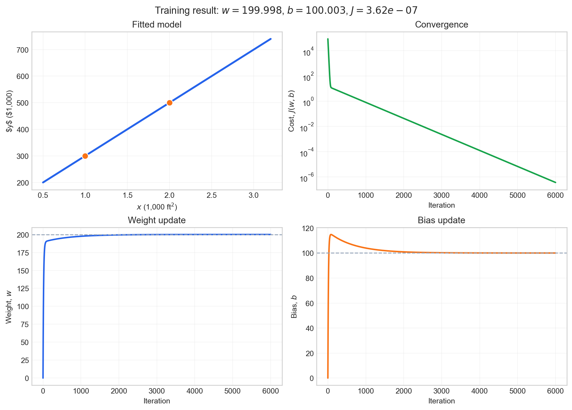
The optimized parameters approach $w=200$ and $b=100$, and the prediction at $x=3$ approaches 700.
5. Choosing a learning rate
The learning rate controls the size of each parameter update.
- If $\alpha$ is too small, training is stable but slow.
- If $\alpha$ is sufficiently large, convergence may be much faster.
- If $\alpha$ is too large, the parameters overshoot the minimum and the cost may diverge.
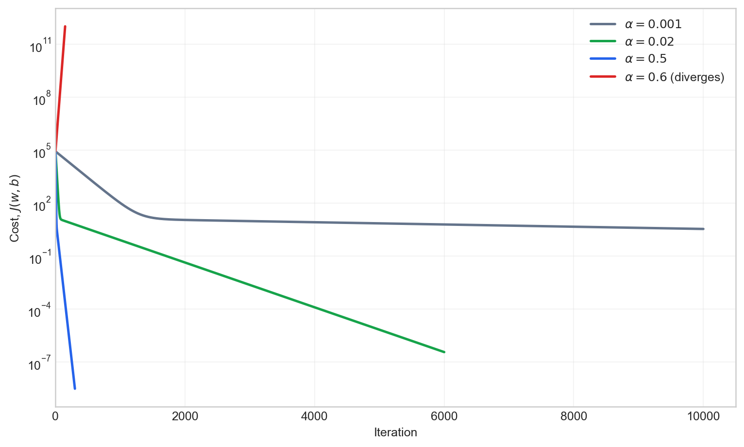
The following comparison uses the same initial parameters, $w=0$ and $b=0$.
| Learning rate | Iterations | Behavior |
|---|---|---|
| 0.001 | 10,000 | Stable but relatively slow |
| 0.02 | 6,000 | Stable and convergent for this dataset |
| 0.5 | 300 | Converges rapidly with oscillation |
| 0.6 | 300 | Diverges |
Interpreting each experiment
With $\alpha=0.001$, the cost falls rapidly at first and then decreases slowly. Ten thousand iterations are not enough to reach the exact solution. This long tail is easy to overlook when only the beginning of the training curve is plotted.
With $\alpha=0.02$, the algorithm makes substantially larger updates while remaining stable. After 6,000 iterations, it obtains approximately
\[w=199.998344,\qquad b=100.002679,\]with $J\approx3.62\times10^{-7}$.
With $\alpha=0.5$, the parameters cross the minimum repeatedly but the oscillations shrink, so the algorithm still converges. A fast result on this two-point dataset does not make 0.5 a safe default for other data.
With $\alpha=0.6$, each overshoot is larger than the previous one. The parameters and cost grow until floating-point arithmetic can no longer represent them reliably. This is divergence rather than slow convergence.
For this particular quadratic objective, the boundary can be examined analytically. The Hessian matrix is
\[H=\frac{1}{m}X^TX= \begin{bmatrix} 2.5 & 1.5\\ 1.5 & 1.0 \end{bmatrix}.\]Its largest eigenvalue is approximately $3.427$. Gradient descent on this quadratic is stable when
\[0<\alpha<\frac{2}{3.427}\approx0.584.\]This calculation explains the experiment: 0.5 lies below the stability boundary, whereas 0.6 lies above it. The boundary changes when the dataset or feature scale changes.
These values are specific to this dataset and its feature scale. They should not be treated as universal defaults. Feature scaling changes the geometry of the cost function and can substantially improve optimization when features have very different numerical ranges.
What this experiment does and does not show
The dataset has only two points and both lie perfectly on one line. It is therefore suitable for tracing the optimization process, but not for evaluating generalization. A cost near zero only confirms that the model fits these training observations. With real data, a separate validation or test set is required to determine whether the learned relationship works for unseen examples.
The experiment also illustrates why preprocessing matters. If house size were measured directly in square feet rather than thousands of square feet, the values of $x$ and the curvature of $J$ would change considerably. The same numerical learning rate could then behave very differently.
In production code, convergence is often detected by monitoring the reduction in cost or the magnitude of the gradient rather than relying only on a fixed iteration count. Storing every parameter state is also unnecessary unless the optimization path is needed for diagnostics or visualization.
6. Complete runnable example
import numpy as np
import matplotlib.pyplot as plt


def predict(x, w, b):
    return w * x + b


def compute_cost(x, y, w, b):
    residuals = predict(x, w, b) - y
    return np.mean(residuals ** 2) / 2


def compute_gradient(x, y, w, b):
    residuals = predict(x, w, b) - y
    return np.mean(residuals * x), np.mean(residuals)


def gradient_descent(x, y, w_init=0.0, b_init=0.0,
                     alpha=0.02, iterations=6_000):
    w = float(w_init)
    b = float(b_init)
    costs = [compute_cost(x, y, w, b)]

    for _ in range(iterations):
        dj_dw, dj_db = compute_gradient(x, y, w, b)
        w -= alpha * dj_dw
        b -= alpha * dj_db
        costs.append(compute_cost(x, y, w, b))

    return w, b, np.asarray(costs)


x_train = np.array([1.0, 2.0])
y_train = np.array([300.0, 500.0])

w, b, costs = gradient_descent(x_train, y_train)

print(f"w={w:.6f}, b={b:.6f}, J={costs[-1]:.3e}")
print(f"Predicted price at x=3: {predict(3.0, w, b):.2f}")

x_line = np.linspace(0.5, 3.2, 200)
fig, axes = plt.subplots(1, 2, figsize=(11, 4))

axes[0].scatter(x_train, y_train, label="training data")
axes[0].plot(x_line, predict(x_line, w, b), label="fitted model")
axes[0].set(xlabel="House size (1,000 ft²)", ylabel="Price (1,000 USD)")
axes[0].legend()

axes[1].semilogy(costs)
axes[1].set(xlabel="Iteration", ylabel="Cost J(w, b)")

plt.tight_layout()
plt.show()
7. Summary
Univariate linear regression represents a continuous target with the model $\hat{y}=wx+b$. Training consists of selecting parameters that minimize a cost function. For the squared-error objective, gradient descent repeatedly computes the partial derivatives with respect to $w$ and $b$ and updates both parameters simultaneously.
The implementation is compact, but the central ideas generalize to larger machine-learning models:
- define a prediction function;
- quantify error with an objective;
- compute the gradient of that objective;
- update parameters with a suitable learning rate;
- verify convergence and evaluate the resulting model.
댓글남기기